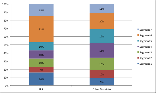
In a previous video, we built a 100% stacked column chart, and added data labels to show actual amounts in an abbreviated custom number format. The result is a chart that shows a proportional breakdown of each quarter by region. Looking at the chart, you might wonder how to show the actual percentages in each bar? This isn't hard to do, but it does take a little prep work. Unlike a pie chart, which has a specific option to show percentages, a 100% stacked chart does not have this option.

But there is an option to pull values from other cells. What this means is that we need to build our own formulas to calculate percentages, then pull these results into the data labels.

To start off, I'll copy and paste the whole table and remove the values. Now to get the right percentage, I need to divide each value in the table above by the total value in the same row, which represents one quarter. In other words, I need to divide C5 by the sum of C5 to F5.

I need to lock this reference carefully.I want the rows to change, but columns need to stay fixed as the formula is being copied across the table. F4 three times will do the job. Now when I copy the formula throughout the table, we get the percentages we need. To add these to the chart, I need select the data labels for each series one at a time, then switch to 'value from cells' under label options. Now we have a 100% stacked chart that shows the percentage breakdown in each column. Whenever you create these kind of helper calculations for a chart, take care with the Switch Column/Row button. If I use it here to group sales by region instead of quarter, the chart looks fine, but the percentages are no longer correct.

Excel indents the data in the column, creating a margin between the data and the adjacent column. Adjust the column width if necessary to accommodate the extra spaces. I have data which ends at the same row but multiple columns in which I want them to be stacked in a sequence where B column data will go under A column data where the data ends for A column and C column data to go under A column data where the data from B column ends and so on.

To fix this problem, I would need to update the formulas in the helper table.

Vpn for mac free trial. How to set up Hotspot Shield VPN for macOS devices Download and install Hotspot Shield VPN by following the instructions. Connect Hotspot Shield VPN in one easy click. Enjoy secure, private browsing from over 2,500 global servers.

What I am assuming is that you have a large worksheet with gaps you need to close up, and that a simple sort would disrupt the order of your data. Here's how I would do it: First add two new temporary columns, new A and new B. Select the range of cells in A from the first all the way to the last row you know has data. Use Edit > Fill > Series > Linear and number them from 1 to whatever. In the next column select the first cell and enter a formula that checks to see if the cells to its right are empty. It could be as simple as adding them all up ( =SUM(C1:K1)) to see if they are zero or it could be a function of logic ( =AND(ISBLANK(C1), ISBLANK(D1)), etc.).

Mail is simple and not that complicated, and the resulting lack of complexity makes it more approachable. Creating rules or email signatures within Mail doesn’t induce knee-knocking anxiety, the way doing so might in, say, Microsoft Outlook.

Copy and paste this formula down all the cells in column B to the end of your range. Now you have two keys with which to sort your worksheet. Sort on column B to find your empty rows and delete them en masse, then restore your worksheet's original sort order by sorting on the first column.